39 modify legend labels excel 2013

Excel Charts with Dynamic Title and Legend Labels Let's create a chart with dynamic title and labels Creating the chart is really simple. Select an empty cell in the worksheet and create an XY chart (scatter with smooth lines). Open the Select Data Source dialog box ( Chart Tools (Design) -> Data -> Select Data ). Click on the Add button to add Legend Entries (Series). How To Change The Horizontal Axis Labels In Excel Right-click the category labels you lot want to change, and click Select Data. In the Horizontal (Category) Centrality Labels box, click Edit. In the Centrality characterization range box, enter the labels yous want to use, separated past commas. For example, type Quarter 1 ,Quarter 2,Quarter three,Quarter 4.

Use defined names to automatically update a chart range - Office Select cells A1:B4. On the Insert tab, click a chart, and then click a chart type. Click the Design tab, click the Select Data in the Data group. Under Legend Entries (Series), click Edit. In the Series values box, type =Sheet1!Sales, and then click OK. Under Horizontal (Category) Axis Labels, click Edit.

Modify legend labels excel 2013

Custom Excel number format - Ablebits.com To create a custom Excel format, open the workbook in which you want to apply and store your format, and follow these steps: Select a cell for which you want to create custom formatting, and press Ctrl+1 to open the Format Cells dialog. Under Category, select Custom. Type the format code in the Type box. Click OK to save the newly created format. How to Change the X-Axis in Excel - Alphr Open the Excel file and select your graph. Now, right-click on the Horizontal Axis and choose Format Axis… from the menu. Select Axis Options > Labels. Under Interval between labels, select the... How to Edit Pie Chart in Excel (All Possible Modifications) As a result, there will be a new ribbon named Format Data Labels at the right side of your Excel file. Now, go to the Label Options menu >> Label Options group >> put a tick mark on the Percentage option. As a result, there will be percentage values too at the data labels. The result sheet would look like this. 👇 9.

Modify legend labels excel 2013. How to Change the Y Axis in Excel - Alphr Go to "Design," then go to "Add Chart Element" and "Axes." You'll have two options: "Primary Horizontal" will hide/unhide the horizontal axis, and if you choose "Primary Vertical," it will... Scatterplot Legend - excelforum.com For a new thread (1st post), scroll to Manage Attachments, otherwise scroll down to GO ADVANCED, click, and then scroll down to MANAGE ATTACHMENTS and click again. Now follow the instructions at the top of that screen. New Notice for experts and gurus: Align Chart Title in Excel - Explained! - ANALYSISTABS.COM The following step by step approach will help you to align the chart title position in the Excel Charts. Align Chart Title in Excel - Step 1: Select a Chart title You can activate any chart and select the chart title to re position the title. The below screen shot will show you how to select the chart title. Format and align chart title Make Excel charts primary and secondary axis the same scale These series may be hard to see so the easiest way to customise them is to click on the Chart, click on the Format tab, and find the series called Primary Scale. Just below this dropdown you can click on Format Selection. On the resultant options box, change the fill to No Fill and the Border to No line. You will do the same for the other new ...

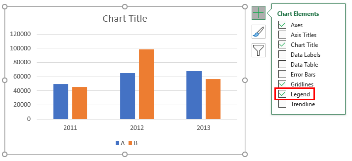
Two Ways To Add a Legend in Excel (With Tips and FAQ) Method one. The first method you can use to add a legend is: Click on your chart: This generates three buttons near the top-right of the chart you can use to adjust your chart. Select the "Chart Elements" button: This button is the top one and looks like a plus sign. Click the box next to "Legend": This auto-generates a legend based on all the ... Controlling Chart Gridlines (Microsoft Excel) In the Current Selection group, use the drop-down list to choose the gridlines you want to control. Click the Format Selection tool, also within the Current Selection group. Excel displays a Format task pane at the right side of the program window. Use the controls in the task pane to make changes to the gridlines, as desired. Close the task pane. Solved: How to create dynamic column headers & custom cond ... - Power BI Column Headers. In Excel, there are always only 13 data columns for each table, the furthest right being the start of the current month (e.g., 01/10/2021), using a formula. The 12 columns then each have EDATE (column-to-right, -1) so that eventually I have a table that always contains the previous 13 rolling months as headers. Format Chart Axis in Excel - Axis Options Remove the unit of the label from the chart axis. The logarithm scale will convert the axis values as a function of the log. reverse the order of chart axis values/ Axis Options: Tick Marks and Labels. Tick marks are the small, marks on the axis for each of the axis values and the sub-divisions that make the chart easier to read.

Custom Chart Data Labels In Excel With Formulas Follow the steps below to create the custom data labels. Select the chart label you want to change. In the formula-bar hit = (equals), select the cell reference containing your chart label's data. In this case, the first label is in cell E2. Finally, repeat for all your chart laebls. Charts in Access - Overview, Instructions, and Video Lesson How to Create a Microsoft Graph Chart in Access. To insert an older, Microsoft Graph chart control into a report in Access, click the "Insert Chart" button in the scrollable list of controls in the "Controls" button group on the "Design" tab of the "Report Design Tools" contextual tab in the Ribbon. Then click and drag over the ... How to Change the Style of Table Titles and Figure Captions in ... Figure 1. Home tab. Select the text of an existing table title or figure caption. Figure 2. Selected table title. Select the dialog box launcher in the Styles group. Figure 3. Styles group dialog box launcher. Select the menu arrow to the right of Caption in the Styles pane. How to add legend title in Excel chart - Data Cornering Go to the Insert tab, and on the right side will be a text box. Selec and draw it over the place where you want it in the chart. If you want the text in the same formatting as in the legend, try format painter. Select legend, click on format painter, and then on the text box. As a result, here is my Excel chart with added legend title.

Excel 2003: Formatting a Chart

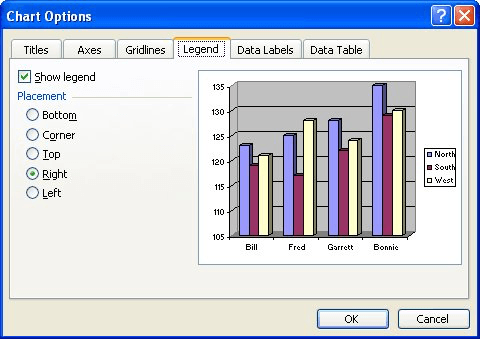
Formatting the Border of a Legend (Microsoft Excel) To change the appearance of the legend's border, follow these steps: Click once on the legend to select it. Handles should appear around the perimeter of the legend. Choose Selected Legend from the Format menu. Excel displays the Format Legend dialog box. Make sure the Patterns tab is selected. (See Figure 1.) Figure 1.

PPT - Tutorial 4 Analyzing and Charting Financial Data PowerPoint Presentation - ID:6169550

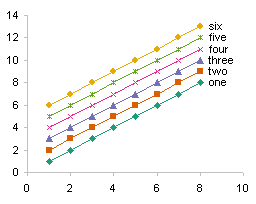
Tutorial on Chart Legend | CanvasJS JavaScript Charts Enabling Default Legend. When we want Legend to appear for a dataSeries, we set showInLegend to true in that dataSeries, this makes the dataSeries to appear in legend. This way you can choose which dataSeries to show in legend. By default name of series is shown in legend. To Customize the text, you can mention legendText in dataSeries.

Unit 4: Charting | Information Systems

Excel Waterfall Chart: How to Create One That Doesn't Suck If your data has a different number of categories, you have to modify the template, which again requires additional work. Ideally, you would create a waterfall chart the same way as any other Excel chart: (1) click inside the data table, (2) click in the ribbon on the chart you want to insert. ... in Excel 2016

Excel Charts with Dynamic Title and Legend Labels | ExcelDemy

Chart.Legend property (Excel) | Microsoft Docs Returns a Legend object that represents the legend for the chart. Read-only. Syntax expression. Legend expression A variable that represents a Chart object. Example This example turns on the legend for Chart1 and then sets the legend font color to blue. VB Charts ("Chart1").HasLegend = True Charts ("Chart1").Legend.Font.ColorIndex = 5

Turning the Legend On and Off (Microsoft Excel)

How to Add Axis Titles in a Microsoft Excel Chart First, right-click an axis title to display the floating toolbar. You'll see options for Style, Fill, and Outline. Use the drop-down arrows next to any of these options to apply a theme, use a gradient or texture, or choose a border style and color. To take your customization a bit further, start by opening the Format Axis Title sidebar.

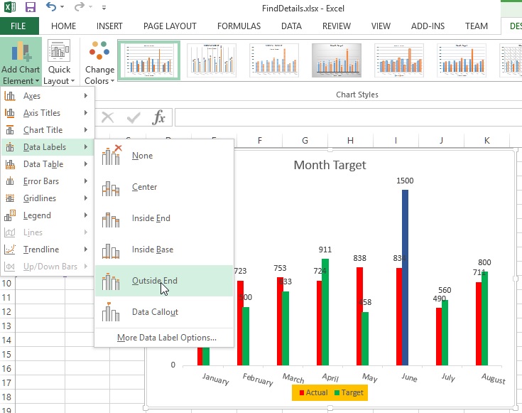
Chart axes, legend, data labels, trendline in Excel - Tech Funda

How to ☝️ Add, Format, and Remove a Chart Legend in Excel Click on the legend. 2. Select the Design tab. 3. Pick the Add Chart Element option. 4. Choose Legend. 5. Click on the type of legend you set before (based on its position), and this will automatically remove it from your Excel chart.

How to Make a Chart or Graph in Excel [With Video Tutorial]

How to Print Labels from Excel - Lifewire Select Mailings > Write & Insert Fields > Update Labels . Once you have the Excel spreadsheet and the Word document set up, you can merge the information and print your labels. Click Finish & Merge in the Finish group on the Mailings tab. Click Edit Individual Documents to preview how your printed labels will appear. Select All > OK .

34 How To Label Legend In Excel - Labels Design Ideas 2020

Adjusting the Order of Items in a Chart Legend (Microsoft Excel) Another way to change the order of the data series (and thus affect the legend) is to right-click any element of the chart (including the legend) to display a Context menu. Click the Select Data option and Excel displays the Select Data Source dialog box. (See Figure 1.) Figure 1. The Select Data Source dialog box.

Understand the Legend and Legend Key in Excel Spreadsheets

How to Create and Customize a Treemap Chart in Microsoft Excel For fill and line styles and colors, effects like shadow and 3-D, or exact size and proportions, you can use the Format Chart Area sidebar. Either right-click the chart and pick "Format Chart Area" or double-click the chart to open the sidebar. On Windows, you'll see two handy buttons on the right of your chart when you select it.

How to Use Charts and Diagrams in Microsoft Excel 2013 | UniversalClass

Excel Chart VBA - 33 Examples For Mastering Charts in Excel VBA The following Excel Chart VBA Examples works similarly when we select some data and click on charts from Insert Menu and to create a new chart. This will create basic chart in an existing worksheet. Sub ExAddingNewChartforSelectedData_Sapes_AddChart_Method () Range ("C5:D7").Select ActiveSheet.Shapes.AddChart.Select End Sub 2.

Directly Labeling Excel Charts - PolicyViz

How to Edit Pie Chart in Excel (All Possible Modifications) As a result, there will be a new ribbon named Format Data Labels at the right side of your Excel file. Now, go to the Label Options menu >> Label Options group >> put a tick mark on the Percentage option. As a result, there will be percentage values too at the data labels. The result sheet would look like this. 👇 9.

Legends in Excel Charts - Formats, Size, Shape, and Position - Peltier Tech Blog

How to Change the X-Axis in Excel - Alphr Open the Excel file and select your graph. Now, right-click on the Horizontal Axis and choose Format Axis… from the menu. Select Axis Options > Labels. Under Interval between labels, select the...