40 show data labels excel
Chart.ApplyDataLabels method (Excel) | Microsoft Docs The type of data label to apply. True to show the legend key next to the point. The default value is False. True if the object automatically generates appropriate text based on content. For the Chart and Series objects, True if the series has leader lines. Pass a Boolean value to enable or disable the series name for the data label. Display every "n" th data label in graphs - Microsoft Community With this tool you can assign a range of cells to be the labels for chart series, instead of the Excel defaults. Using a formula, you can have a text show up in every nth cell and then use that range with the XY Chart Labeler to display as the series label. If the full chart labels are in column A, starting in cell A1, then you can use this ...
How to use data labels in a chart - YouTube Excel charts have a flexible system to display values called "data labels". Data labels are a classic example a "simple" Excel feature with a huge range of o...

Show data labels excel
How to add data labels from different column in an Excel chart? Right click the data series, and select Format Data Labels from the context menu. 3. In the Format Data Labels pane, under Label Options tab, check the Value From Cells option, select the specified column in the popping out dialog, and click the OK button. Now the cell values are added before original data labels in bulk. 4. How to Add Data Labels to an Excel 2010 Chart - dummies On the Chart Tools Layout tab, click Data Labels→More Data Label Options. The Format Data Labels dialog box appears. You can use the options on the Label Options, Number, Fill, Border Color, Border Styles, Shadow, Glow and Soft Edges, 3-D Format, and Alignment tabs to customize the appearance and position of the data labels. › documents › excelHow to show percentages in stacked column chart in Excel? 1. Select data range you need and click Insert > Column > Stacked Column. See screenshot: 2. Click at the column and then click Design > Switch Row/Column. 3. In Excel 2007, click Layout > Data Labels > Center. In Excel 2013 or the new version, click Design > Add Chart Element > Data Labels > Center. 4.
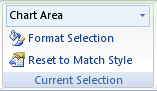
Show data labels excel. chandoo.org › wp › change-data-labels-in-chartsHow to Change Excel Chart Data Labels to Custom Values? May 05, 2010 · Now, click on any data label. This will select “all” data labels. Now click once again. At this point excel will select only one data label. Go to Formula bar, press = and point to the cell where the data label for that chart data point is defined. Repeat the process for all other data labels, one after another. See the screencast. Format Data Labels in Excel- Instructions - TeachUcomp, Inc. To do this, click the "Format" tab within the "Chart Tools" contextual tab in the Ribbon. Then select the data labels to format from the "Chart Elements" drop-down in the "Current Selection" button group. Then click the "Format Selection" button that appears below the drop-down menu in the same area. Data label name appear on hover - excelforum.com For a new thread (1st post), scroll to Manage Attachments, otherwise scroll down to GO ADVANCED, click, and then scroll down to MANAGE ATTACHMENTS and click again. Now follow the instructions at the top of that screen. New Notice for experts and gurus: Add or remove data labels in a chart - support.microsoft.com Right-click the data series or data label to display more data for, and then click Format Data Labels. Click Label Options and under Label Contains, select the Values From Cells checkbox. When the Data Label Range dialog box appears, go back to the spreadsheet and select the range for which you want the cell values to display as data labels.
how to add data labels into Excel graphs - storytelling with data You can download the corresponding Excel file to follow along with these steps: Right-click on a point and choose Add Data Label. You can choose any point to add a label—I'm strategically choosing the endpoint because that's where a label would best align with my design. Excel defaults to labeling the numeric value, as shown below. How to show data label in "percentage" instead of - Microsoft Community Select Format Data Labels Select Number in the left column Select Percentage in the popup options In the Format code field set the number of decimal places required and click Add. (Or if the table data in in percentage format then you can select Link to source.) Click OK Regards, OssieMac Report abuse 8 people found this reply helpful · How to add text labels on Excel scatter chart axis - Data Cornering Add dummy series to the scatter plot and add data labels. 4. Select recently added labels and press Ctrl + 1 to edit them. Add custom data labels from the column "X axis labels". Use "Values from Cells" like in this other post and remove values related to the actual dummy series. Change the label position below data points. DataLabels.ShowValue property (Excel) | Microsoft Docs This example enables the value to be shown for the data labels of the first series, on the first chart. This example assumes that a chart exists on the active worksheet. VB Copy Sub UseValue () ActiveSheet.ChartObjects (1).Activate ActiveChart.SeriesCollection (1) _ .DataLabels.ShowValue = True End Sub Support and feedback
Excel charts: how to move data labels to legend - Microsoft Tech Community Excel charts: how to move data labels to legend ... You can't do that, but you can show a data table below the chart instead of data labels: Click anywhere on the chart. On the Design tab of the ribbon (under Chart Tools), in the Chart Layouts group, click Add Chart Element > Data Table > With Legend Keys (or No Legend Keys if you prefer) ... › blog › 2021A Comprehensive guide to Microsoft Excel for Data Analysis Nov 24, 2021 · You can make a chart, modify its type, adjust the row or column, the legend location, and the data labels. Column Chart, Line Chart, Pie Chart, Bar Chart, Area Chart, Scatter Plot are some of the different types of charts provided in Microsoft Excel. 10) Data Validation. Only valid values may need to be entered into cells. support.microsoft.com › en-us › officePrepare your Excel data source for a Word mail merge Step 1: Set up your data source in Excel. If you're using an Excel spreadsheet as your data source for a mail merge in Word, skip this step. If the data source is a .txt or a .csv file, use the Text Import Wizard to set up your data in Excel. After you successfully import a .txt or .csv file, go to Step 2. Add data labels and callouts to charts in Excel 365 - EasyTweaks.com Step #1: After generating the chart in Excel, right-click anywhere within the chart and select Add labels . Note that you can also select the very handy option of Adding data Callouts. Step #2: When you select the "Add Labels" option, all the different portions of the chart will automatically take on the corresponding values in the table ...

How to sort data with Microsoft Excel 2016 - MATC Information Technology Programs: Degrees ...
How to create Custom Data Labels in Excel Charts Click on the Plus sign next to the chart and choose the Data Labels option. We do NOT want the data to be shown. To customize it, click on the arrow next to Data Labels and choose More Options … Unselect the Value option and select the Value from Cells option. Choose the third column (without the heading) as the range.
Chart's Data Series in Excel - Easy Excel Tutorial
How to Add Data Labels in Excel - Excelchat | Excelchat After inserting a chart in Excel 2010 and earlier versions we need to do the followings to add data labels to the chart; Click inside the chart area to display the Chart Tools. Figure 2. Chart Tools. Click on Layout tab of the Chart Tools. In Labels group, click on Data Labels and select the position to add labels to the chart.

How to Add Data Labels in Excel - Excelchat | Excelchat
› xlpivot05How to Control Excel Pivot Table with Field Setting Options Jul 10, 2021 · Check the 'Show items with no data' check box. Click OK; Show all the data in Excel 2003. Make the following change for each field in which you want to see all the data: Double-click the field button, to open the PivotTable field dialog box. Check the 'Show items with no data' check box. Click OK; Missing Data in Pivot Table

How to select best Excel Charts for Data Analysis & Reporting
How to Add Labels to Scatterplot Points in Excel - Statology Step 3: Add Labels to Points Next, click anywhere on the chart until a green plus (+) sign appears in the top right corner. Then click Data Labels, then click More Options… In the Format Data Labels window that appears on the right of the screen, uncheck the box next to Y Value and check the box next to Value From Cells.
Add or remove data labels in a chart - Office Support
How To Add Data Labels In Excel . Adopteesearch July Right click the data series in the chart, and select add data labels > add data labels from the context menu to add data labels. Click on each unwanted label (using slow double click) and delete it. Click finish & merge in the finish group on the mailings tab. Press f2 to move focus to the formula editing box.
Post a Comment for "40 show data labels excel"