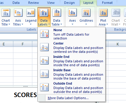
44 excel graph data labels
Change the format of data labels in a chart To get there, after adding your data labels, select the data label to format, and then click Chart Elements > Data Labels > More Options. To go to the appropriate area, click one of the four icons ( Fill & Line, Effects, Size & Properties ( Layout & Properties in Outlook or Word), or Label Options) shown here. Bar Graph in Excel — All 4 Types Explained Easily - Simon Sez IT There are actually 4 types of bar graphs available in Excel. Simple bar graph which shows bars of data for one variable. Grouped bar graph which shows bars of data for multiple variables. Stacked bar graph which shows the contribution of each variable to the total. Percentage bar graph which shows the percentage of contribution to the total.
How to I rotate data labels on a column chart so that they are ... To change the text direction, first of all, please double click on the data label and make sure the data are selected (with a box surrounded like following image). Then on your right panel, the Format Data Labels panel should be opened. Go to Text Options > Text Box > Text direction > Rotate

Excel graph data labels
how to add data labels into Excel graphs - storytelling with data You can download the corresponding Excel file to follow along with these steps: Right-click on a point and choose Add Data Label. You can choose any point to add a label—I'm strategically choosing the endpoint because that's where a label would best align with my design. Excel defaults to labeling the numeric value, as shown below. How to Change Excel Chart Data Labels to Custom Values? - Chandoo.org May 05, 2010 · Now, click on any data label. This will select “all” data labels. Now click once again. At this point excel will select only one data label. Go to Formula bar, press = and point to the cell where the data label for that chart data point is defined. Repeat the process for all other data labels, one after another. See the screencast. How to format axis labels as thousands/millions in Excel? - ExtendOffice Reuse Anything: Add the most used or complex formulas, charts and anything else to your favorites, and quickly reuse them in the future. More than 20 text features: Extract Number from Text String; Extract or Remove Part of Texts; Convert Numbers and Currencies to English Words. Merge Tools: Multiple Workbooks and Sheets into One; Merge Multiple Cells/Rows/Columns Without Losing Data; Merge ...
Excel graph data labels. 3 Axis Graph Excel Method: Add a Third Y-Axis - EngineerExcel Scale the Data for an Excel Graph with 3 Variables. ... Add Data Labels To a Multiple Y-Axis Excel Chart. Axis labels were created by right-clicking on the series and selecting “Add Data Labels”. By default, Excel adds the y-values of the data series. In this case, these were the scaled values, which wouldn’t have been accurate labels for ... TOP 9 what are data labels in excel BEST and NEWEST - Kiến Thức Về ... 7.Data Labels in Excel Pivot Chart (Detailed Analysis) - ExcelDemy. Author: . Post date: 10 yesterday. Rating: 5 (342 reviews) Highest rating: 5. Low rated: 2. Summary: Here, we change the appearances, and background, dynamic data label shows percentages/cell values as data labels in the Pivot chart in Excel. Prevent Overlapping Data Labels in Excel Charts - Peltier Tech May 24, 2021 · Overlapping Data Labels. Data labels are terribly tedious to apply to slope charts, since these labels have to be positioned to the left of the first point and to the right of the last point of each series. ... Loop through every graph in the active workbook ‘SOURCE: ... An internet search of “excel vba overlap data labels” will find you ... Excel Charts - Aesthetic Data Labels - tutorialspoint.com Data Label Positions. To place the data labels in the chart, follow the steps given below. Step 1 − Click the chart and then click chart elements. Step 2 − Select Data Labels. Click to see the options available for placing the data labels. Step 3 − Click Center to place the data labels at the center of the bubbles.
How to Add Labels to Scatterplot Points in Excel - Statology Step 3: Add Labels to Points. Next, click anywhere on the chart until a green plus (+) sign appears in the top right corner. Then click Data Labels, then click More Options…. In the Format Data Labels window that appears on the right of the screen, uncheck the box next to Y Value and check the box next to Value From Cells. Excel charts: how to move data labels to legend @Matt_Fischer-Daly . You can't do that, but you can show a data table below the chart instead of data labels: Click anywhere on the chart. On the Design tab of the ribbon (under Chart Tools), in the Chart Layouts group, click Add Chart Element > Data Table > With Legend Keys (or No Legend Keys if you prefer) How to add data labels from different column in an Excel chart? This method will guide you to manually add a data label from a cell of different column at a time in an Excel chart. 1. Right click the data series in the chart, and select Add Data Labels > Add Data Labels from the context menu to add data labels. 2. How to change Axis labels in Excel Chart - A Complete Guide Right-click the horizontal axis (X) in the chart you want to change. In the context menu that appears, click on Select Data…. A Select Data Source dialog opens. In the area under the Horizontal (Category) Axis Labels box, click the Edit command button. Enter the labels you want to use in the Axis label range box, separated by commas.
How to create Custom Data Labels in Excel Charts - Efficiency 365 Create the chart as usual. Add default data labels. Click on each unwanted label (using slow double click) and delete it. Select each item where you want the custom label one at a time. Press F2 to move focus to the Formula editing box. Type the equal to sign. Now click on the cell which contains the appropriate label. Add or remove data labels in a chart - support.microsoft.com Add data labels to a chart Click the data series or chart. To label one data point, after clicking the series, click that data point. In the upper right corner, next to the chart, click Add Chart Element > Data Labels. To change the location, click the arrow, and choose an option. Find, label and highlight a certain data point in Excel scatter graph Oct 10, 2018 · Select the Data Labels box and choose where to position the label. By default, Excel shows one numeric value for the label, y value in our case. To display both x and y values, right-click the label, click Format Data Labels…, select the X Value and Y value boxes, and set the Separator of your choosing: Label the data point by name Linking a graph in PowerPoint to the Excel data so the graph can ... Follow the same procedure each month for copying the cells from the current version of the Excel file to the data table for the graph on the appropriate slides. Then, update either a text box on the slide or the Slide Notes with the date and time of the update and the file name the data came from. ... Set all legends, labels, axes, gridlines ...
How to Data Labels in a Line Graph in Excel 2007 - YouTube
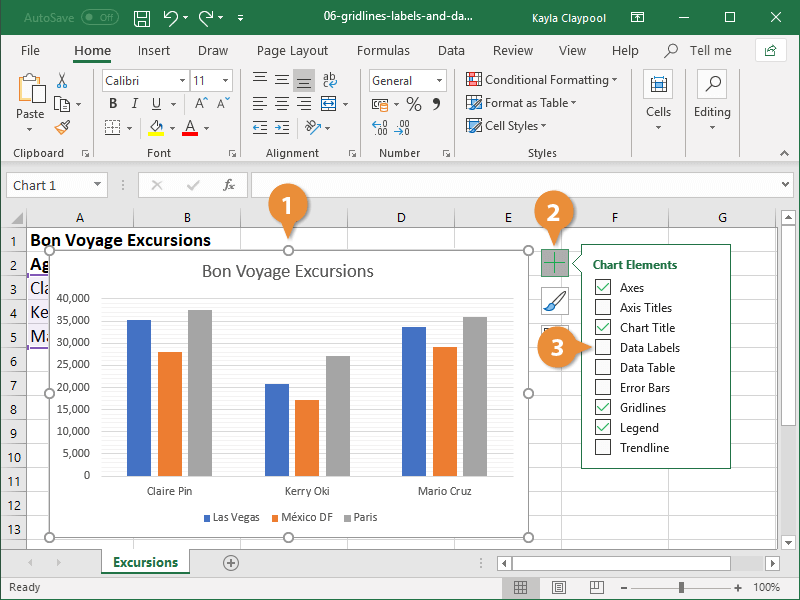
How to add or move data labels in Excel chart? - ExtendOffice In Excel 2013 or 2016. 1. Click the chart to show the Chart Elements button . 2. Then click the Chart Elements, and check Data Labels, then you can click the arrow to choose an option about the data labels in the sub menu. See screenshot: In Excel 2010 or 2007. 1. click on the chart to show the Layout tab in the Chart Tools group. See ...

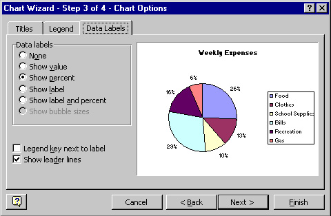
410 How to display percentage labels in pie chart in Excel 2016 - YouTube
Edit titles or data labels in a chart - support.microsoft.com The first click selects the data labels for the whole data series, and the second click selects the individual data label. Right-click the data label, and then click Format Data Label or Format Data Labels. Click Label Options if it's not selected, and then select the Reset Label Text check box. Top of Page

Directly Labeling Excel Charts - PolicyViz
How to create a chart with both percentage and value in Excel? After installing Kutools for Excel, please do as this:. 1.Click Kutools > Charts > Category Comparison > Stacked Chart with Percentage, see screenshot:. 2.In the Stacked column chart with percentage dialog box, specify the data range, axis labels and legend series from the original data range separately, see screenshot:. 3.Then click OK button, and a prompt message is popped out to remind you ...
Charts
Data Labels in Excel Pivot Chart (Detailed Analysis) 7 Suitable Examples with Data Labels in Excel Pivot Chart Considering All Factors 1. Adding Data Labels in Pivot Chart 2. Set Cell Values as Data Labels 3. Showing Percentages as Data Labels 4. Changing Appearance of Pivot Chart Labels 5. Changing Background of Data Labels 6. Dynamic Pivot Chart Data Labels with Slicers 7.

SQL & BI Learning: Pie Chart with data labels outside in ssrs
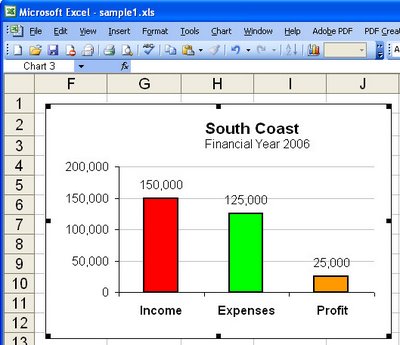
How to make a chart (graph) in Excel and save it as template - Ablebits.com Oct 22, 2015 · 3. Inset the chart in Excel worksheet. To add the graph on the current sheet, go to the Insert tab > Charts group, and click on a chart type you would like to create.. In Excel 2013 and Excel 2016, you can click the Recommended Charts button to view a gallery of pre-configured graphs that best match the selected data.. In this example, we are creating a 3-D …

Chapter 3 Excel 2007/2010 Charts
How to hide zero data labels in chart in Excel? - ExtendOffice If you want to hide zero data labels in chart, please do as follow: 1. Right click at one of the data labels, and select Format Data Labels from the context menu. See screenshot: 2. In the Format Data Labels dialog, Click Number in left pane, then select Custom from the Category list box, and type #"" into the Format Code text box, and click Add button to add it to Type list box.
Data labels on Excel charts « projectwoman.com
Excel: How to Create a Bubble Chart with Labels - Statology Step 3: Add Labels. To add labels to the bubble chart, click anywhere on the chart and then click the green plus "+" sign in the top right corner. Then click the arrow next to Data Labels and then click More Options in the dropdown menu: In the panel that appears on the right side of the screen, check the box next to Value From Cells within ...
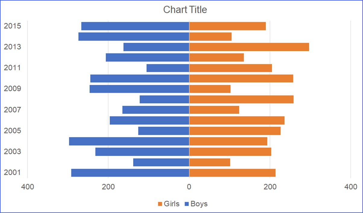
How to Make a Side by Side Comparison Bar Chart - excelnotes.com
How to Add Total Data Labels to the Excel Stacked Bar Chart Apr 03, 2013 · Step 4: Right click your new line chart and select “Add Data Labels” Step 5: Right click your new data labels and format them so that their label position is “Above”; also make the labels bold and increase the font size. Step 6: Right click the line, select “Format Data Series”; in the Line Color menu, select “No line”
How to Add Axis Labels to a Chart in Excel | CustomGuide
How to Make a Bar Graph in Excel: 9 Steps (with Pictures) - wikiHow May 02, 2022 · It's easy to spruce up data in Excel and make it easier to interpret by converting it to a bar graph. A bar graph is not only quick to see and understand, but it's also more engaging than a list of numbers. ... Add labels for the graph's X- and Y-axes. To do so, click the A1 cell (X-axis) and type in a label, ...

charts - Excel, giving data labels to only the top/bottom X% values - Stack Overflow
DataLabels collection (Excel Graph) | Microsoft Docs In this article. A collection of all the DataLabel objects for the specified series. Each DataLabel object represents a data label for a point or trendline. For a series without definable points (such as an area series), the DataLabels collection contains a single data label.. Remarks. Use the DataLabels method to return the DataLabels collection.. Use DataLabels (index), where index is the ...

Adobe Acrobat Standard Help 7.0 Instruction Manual 7 En
Create Dynamic Chart Data Labels with Slicers - Excel Campus Feb 10, 2016 · Step 3: Use the TEXT Function to Format the Labels. Typically a chart will display data labels based on the underlying source data for the chart. In Excel 2013 a new feature called “Value from Cells” was introduced. This feature allows us to specify the a range that we want to use for the labels.
how to make a excel graph. - Computer Notes
Custom Chart Data Labels In Excel With Formulas - How To Excel At Excel Follow the steps below to create the custom data labels. Select the chart label you want to change. In the formula-bar hit = (equals), select the cell reference containing your chart label's data. In this case, the first label is in cell E2. Finally, repeat for all your chart laebls.

Adding custom error bars in Mac Excel 2008 - YouTube
How to format axis labels as thousands/millions in Excel? - ExtendOffice Reuse Anything: Add the most used or complex formulas, charts and anything else to your favorites, and quickly reuse them in the future. More than 20 text features: Extract Number from Text String; Extract or Remove Part of Texts; Convert Numbers and Currencies to English Words. Merge Tools: Multiple Workbooks and Sheets into One; Merge Multiple Cells/Rows/Columns Without Losing Data; Merge ...
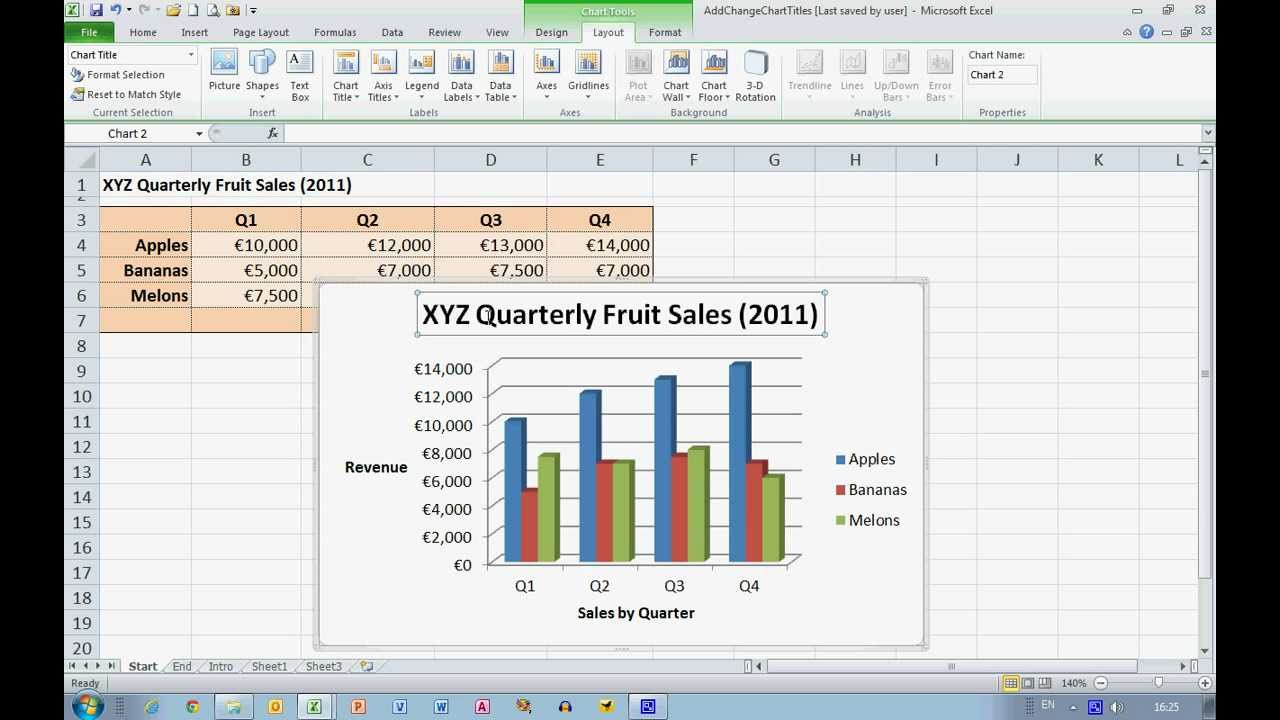
How To... Add and Change Chart Titles in Excel 2010 - YouTube
How to Change Excel Chart Data Labels to Custom Values? - Chandoo.org May 05, 2010 · Now, click on any data label. This will select “all” data labels. Now click once again. At this point excel will select only one data label. Go to Formula bar, press = and point to the cell where the data label for that chart data point is defined. Repeat the process for all other data labels, one after another. See the screencast.

Quickly Create A Variable Width Column Chart In Excel
how to add data labels into Excel graphs - storytelling with data You can download the corresponding Excel file to follow along with these steps: Right-click on a point and choose Add Data Label. You can choose any point to add a label—I'm strategically choosing the endpoint because that's where a label would best align with my design. Excel defaults to labeling the numeric value, as shown below.

How To Use Dynamic Data Labels To Create Interactive Excel Charts
How to Data Labels in a Bar Graph in Excel 2013 - YouTube
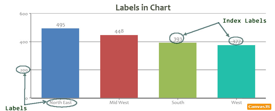
Tutorial on Labels & Index Labels in Chart | CanvasJS JavaScript Charts
Post a Comment for "44 excel graph data labels"